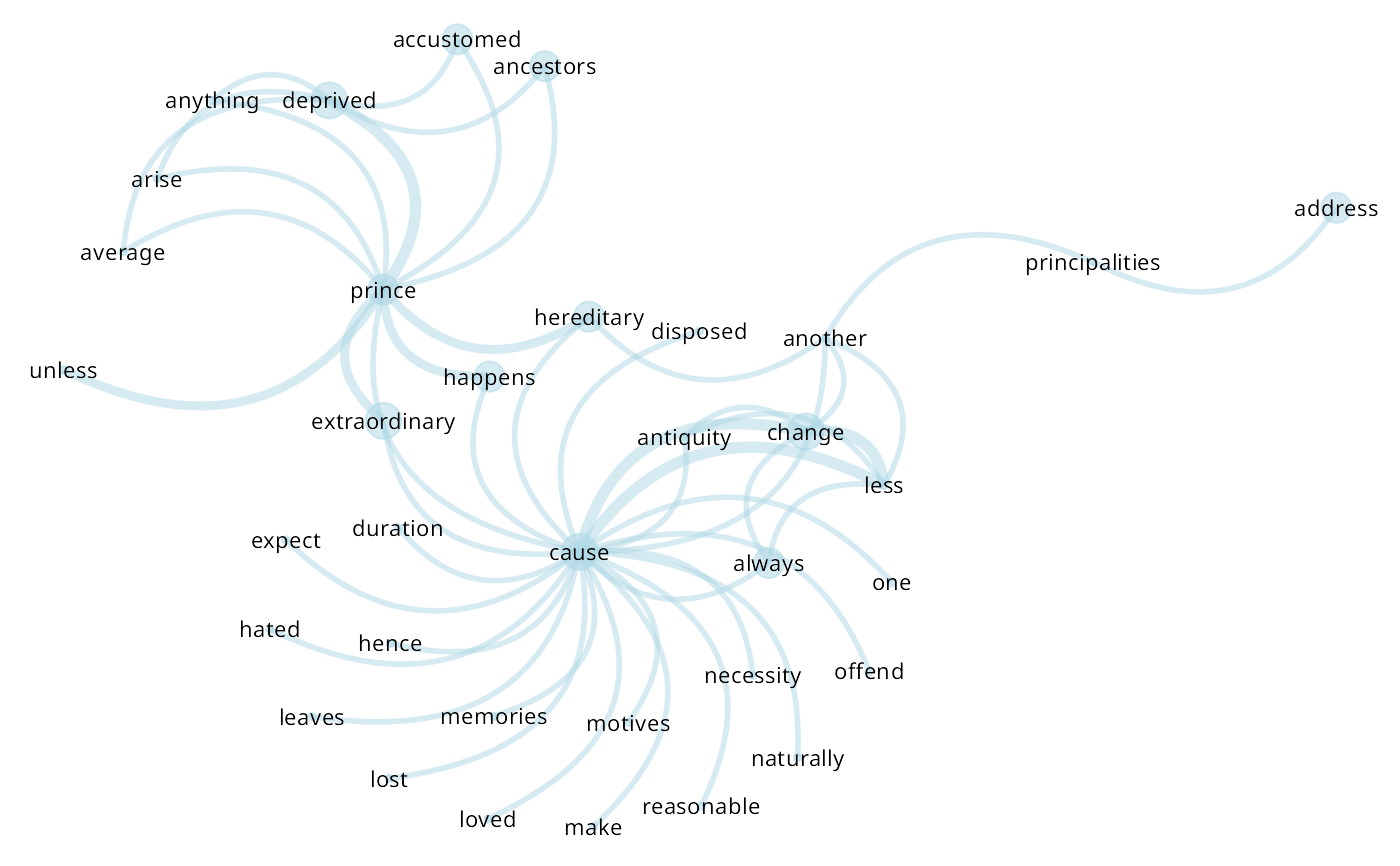
Plot a network of co-occurrence of terms. Because word frequencies can vary significantly, differences in text size can be substantial. Therefore, instead of adjusting text size, we vary the dot/node size, ensuring the text remains consistently sized and maintains readability. It is also possible to normalize the result with log. plot a graph of co-occurrence of terms, as returned by extract_graph, cooccur
Usage
plot_graph2(
  DF,
  text,
  head_n = 30,
  lower = TRUE,
  text_color = "black",
  text_size = 3,
  text_contour_color = NA,
  node_alpha = 0.5,
  node_color = NULL,
  node_size = NULL,
  edge_color = "lightblue",
  edge_alpha = 0.5,
  edge_cut = 0,
  edge_type = "arc",
  edge_bend = 0.5,
  edge_fan = FALSE,
  scale_graph = "scale_values",
  layout = "kk"
)
Arguments
- DF
a dataframe of co-occurrence, extracted with `extract_graph()` and `count(n1, n2)`
- text
an input text
- head_n
number of nodes to show - the more frequent
- lower
Convert words to lowercase. If the text is passed in all lowercase, it can return false sentence and paragraph tokenization.
- text_color
color of the text in nodes
- text_size
font size of the nodes. If empty (default), it will use the frequency of word.
- node_alpha
transparency of the nodes
- node_color
color of the nodes. If empty (default), it will use the same color of the edges.
- edge_color
color of the edges
- edge_alpha
transparency of the edges. Values between 0 and 1.
- edge_cut
in mm, how much you want that the edge stop before reach the node. Can improve readability.
- edge_fan
if TRUE, the edges are drawn in a fan shape. Default FALSE.
- scale_graph
name of a function to normalize the result. Sometimes, the range of numbers are so wide that the graph becomes unreadable. Applying a function to normalize the result can improve the readability, for example using `scale_graph = "log2"`, `"sqrt"`,`"log10"` or `none`.
- layout
the layout of the plot. Options are bipartite, star, circle, nicely, dh, gem, graphopt, grid, mds, sphere, randomly, fr, kk, drl, lgl. More info at ggraph documentation
Examples
text <- ex_prince[3, 2]
graph <- cooccur_words(text, sw = stopwords::stopwords())
#> tokenizing sentences...
#> tokenizing words...
plot_graph2(DF = graph, text = text, head_n = 50, scale_graph = "log2")
#>
  |
  |                                                                      |   0%
  |
  |==                                                                    |   3%
  |
  |====                                                                  |   6%
  |
  |======                                                                |   9%
  |
  |========                                                              |  11%
  |
  |==========                                                            |  14%
  |
  |============                                                          |  17%
  |
  |==============                                                        |  20%
  |
  |================                                                      |  23%
  |
  |==================                                                    |  26%
  |
  |====================                                                  |  29%
  |
  |======================                                                |  31%
  |
  |========================                                              |  34%
  |
  |==========================                                            |  37%
  |
  |============================                                          |  40%
  |
  |==============================                                        |  43%
  |
  |================================                                      |  46%
  |
  |==================================                                    |  49%
  |
  |====================================                                  |  51%
  |
  |======================================                                |  54%
  |
  |========================================                              |  57%
  |
  |==========================================                            |  60%
  |
  |============================================                          |  63%
  |
  |==============================================                        |  66%
  |
  |================================================                      |  69%
  |
  |==================================================                    |  71%
  |
  |====================================================                  |  74%
  |
  |======================================================                |  77%
  |
  |========================================================              |  80%
  |
  |==========================================================            |  83%
  |
  |============================================================          |  86%
  |
  |==============================================================        |  89%
  |
  |================================================================      |  91%
  |
  |==================================================================    |  94%
  |
  |====================================================================  |  97%
  |
  |======================================================================| 100%
#> Using node_size proportional to word frequency as no node_size was provided in parameters