01 Networds - a package to extract and plot words and entities network
Source:vignettes/networds_package.Rmd
networds_package.RmdAbstract
Networds is a package to extract networks from texts. It can extract co-occurrence of words, pattern of words, of entities. It also has bult-in visualization tools.The amount of information nowadays growth exponentially. To capture meaning from huge amount of text is a challenge. Nowadays there is a lot of options with Large Language Models, but this option here is a deterministic one. One possibility to help with this problem of meaning extraction is the use of networks of words and entities. It is called with many different names, such as “semantic networks”, “co-occurrence networks”, “word networks”.
As any other NLP tool, it do not replace the necessity of close reading, but reduce this necessity to read everything, guiding the reading to what the researcher really think is important.
It is better to capture the meaning, when there is a small amount of texts. So, having a huge text, it is possible to choose some target words, re-filter the text with this words, and re-generate the semantic network.
Semantic Networks
Begin extracting using NER and word cooccurrence If you go to check the entities you extracted, maybe word cooccurrence will be better, since extract entities will not
Traditional word tokenizers, like
tokenizers::tokenize_by_words() in the case of URLs, it can
make a mess, so networds has its own word tokenizer to avoid it.
txt <- "Take look at our website https::www/example.org/complement=?foobar123"
# the normal tokenizer used in many packages
txt |> tokenizers::tokenize_words()
#> [[1]]
#>  [1] "take"        "look"        "at"          "our"         "website"
#>  [6] "https"       "www"         "example.org" "complement"  "foobar123"
# the tokenizer of networds
txt |> networds::tokenize_by_words()
#> [[1]]
#> [1] "take"
#> [2] "look"
#> [3] "at"
#> [4] "our"
#> [5] "website"
#> [6] "https::www/example.org/complement=foobar123"
After extracting the nodes, they are sorted alphabetically in the dataframe. So if the phrase is “lorem ipsum”, the nodes will be Col1:“ipsum” and col2:“lorem” instead of the original col1:“lorem” col2:“ipsum”. The reason to that is to ensure that a word pair is always counted in the same way, avoiding that pairs like A-B and B-A be counted as different nodes.
cooccur_words("lorem ipsum. Ipsum lorem")
#> tokenizing sentences...
#> tokenizing words...
#> # A tibble: 1 × 3
#>   n1    n2        n
#>   <chr> <chr> <int>
#> 1 ipsum lorem     2
Collocation.
After running network, some pairs can indicate that there is a
compounded word there. One tip to give a better analysis and
visualization is to treat it as one word, and we can do it by replacing
the white space between the words using a underline. To make multiple
substitutions, use a named vector in str_replace_all, or
transform a dataframe into one by using deframe:
dictionay_of_substitutions <- tibble::tribble(
  ~from, ~to,
  "New York Times", "NYT",
  "New York", "New_York"
)

txt_wiki |>
  stringr::str_replace_all(tibble::deframe(dictionay_of_substitutions)) |>
  dplyr::nth(3) # filtering the 3rd element of vector
#> [1] "Brian Thompson, the 50-year-old CEO of the American health insurance company UnitedHealthcare, was shot and killed in Midtown Manhattan, New_York City, on December 4, 2024. The shooting occurred early in the morning outside an entrance to the New_York Hilton Midtown hotel.[4] Thompson was in the city to attend an annual investors' meeting for UnitedHealth Group, the parent company of UnitedHealthcare. Prior to his death, he faced criticism for the company's rejection of insurance claims, and his family reported that he had received death threats in the past. The suspect, initially described as a white man wearing a mask, fled the scene.[1] On December 9, 2024, authorities arrested 26-year-old Luigi Mangione in Altoona, Pennsylvania, and charged him with Thompson's murder in a Manhattan court.[5][6][7]"
You can have a previous table with, or more wisely, you may run the coocurrence extraction, check if one or some of the most frequent pairs looks like a single word, procede the substitution, check again, and this process again. In the case of proper names It can be not a good idea to do it, since normally surname and name apprears in different proportion, and to consider the prename and surname as a single word will decrease the number of times the surname appears. This process can be made also to reduce some variances of the same word to a common unique case.
Weighting results
It can happens that one pair or a set of pairs appears very frequently and is not representative of the corpus, but comes from a single document can have a set of so repeated pairs that will appear in the network. It is very common problem when dealing with data from social media platforms, like x/Twitter, Reddit, etc. One single user with one single post with repeated pair can make you think a topic is hot when it is not. To avoid it, there is some strategies to weight the nodes and pairs. The simplest is to restrict the number of pairs a document can contribute to the corpus. In networds, we can do it by getting the pair frequency per document, and then making all values above a threshold be flatten.
corpus <- c(
  "I hate you! I hate you! I hate you! I hate you! I hate you! I hate you! I hate you! I hate you! I hate you! I hate you!  I hate you! I hate you! I hate you so much!",
  "Lorem ipsum dolor sit amet, consectetur adipiscing elit.",
  "Nullam pulvinar ante ut elit scelerisque, nec hendrerit orci dapibus. Ut auctor hendrerit dignissim.",
  "Nulla accumsan, lorem non lacinia condimentum, urna dui egestas erat, nec porta urna erat quis elit."
)
# simple coocurrence gives the first doc a great importance
cooccur_words(corpus)
#> You provided a vector of 4 elements instead of one. No problem, but these will be collapsed into a single element, with a final punctuation mark added to each, to ensure it is treated as different sentences in the process of tokenization.
#> tokenizing sentences...
#> tokenizing words...
#> # A tibble: 177 × 3
#>    n1          n2        n
#>    <chr>       <chr> <int>
#>  1 hate        i        13
#>  2 hate        you      13
#>  3 i           you      13
#>  4 erat        urna      4
#>  5 accumsan    erat      2
#>  6 accumsan    urna      2
#>  7 condimentum erat      2
#>  8 condimentum urna      2
#>  9 dui         erat      2
#> 10 dui         urna      2
#> # ℹ 167 more rows
# word coocurrence per document instead of per corpus
cooc <- corpus |>
  cooccur_words(output = "df2")
#> tokenizing sentences...
#> tokenizing words...
#> Each vector element will be considered as a different document. The frequency of co-occurrence per document takes much more time than per corpus.
#> Process began at 18:56:22 2026-05-10
#> Binding dataframes
#> ------------------------------
#> Finished in 0 minutes.

threshold <- 1
Option 1:
cooc_parsim <- cooc |>
  networds::reduce_freq(3)

cooc_parsim
#> # A tibble: 177 × 3
#>    n1          n2        n
#>    <chr>       <chr> <dbl>
#>  1 erat        urna      3
#>  2 hate        i         3
#>  3 hate        you       3
#>  4 i           you       3
#>  5 accumsan    erat      2
#>  6 accumsan    urna      2
#>  7 condimentum erat      2
#>  8 condimentum urna      2
#>  9 dui         erat      2
#> 10 dui         urna      2
#> # ℹ 167 more rows
Option 2, doing the same manually:
cooc_parsim <- cooc |>
  mutate(n = ifelse(n > threshold, threshold, n))

cooc_parsim2 <- cooc_parsim |>
  dplyr::group_by(n1, n2) |>
  dplyr::summarize(n = sum(n)) |>
  dplyr::arrange(dplyr::desc(n))
#> `summarise()` has regrouped the output.
#> ℹ Summaries were computed grouped by n1 and n2.
#> ℹ Output is grouped by n1.
#> ℹ Use `summarise(.groups = "drop_last")` to silence this message.
#> ℹ Use `summarise(.by = c(n1, n2))` for per-operation grouping
#>   (`?dplyr::dplyr_by`) instead.
Visualization
When filtering a text using a keyword and building a graph from that, very often it leads to a high centrality of that very term, in a star shape network. To improve readability, a common practice is to delete from network that term or terms used in filter.
To filter both nodes, there is two options:
filter_graph, that filter exact matches, and
filter_graph_g, that uses grep and regex.
# The package comes with Prince from Machiavelli
Text <- ex_prince$text[1:6]

# stopwords
my_sw <- c("him", "by", "as", "because", "by", "who", "on", "i", "of", "the", "and", "a", "to", "it", "or", "so", "that", "be", "with", "in", "he", "have", "they", "had", "which", "for", "are", "them", "is", "would", "as", "him", "by", "as", "because", "by", "who", "on", "i", "but", "one", "did", "if", "when", "this", "from", "their", "there", "was", "his", "at", "these", "do", "has", "no", "nor", "not", "your", "an", "those", "will", "were", "been", "himself", "themselves") |>
  sort() |>
  unique()

cooc <- cooccur_words(Text, my_sw)
#> You provided a vector of 6 elements instead of one. No problem, but these will be collapsed into a single element, with a final punctuation mark added to each, to ensure it is treated as different sentences in the process of tokenization.
#> tokenizing sentences...
#> tokenizing words...

cooc |> filter_graph("prince")
#> # A tibble: 401 × 3
#>    n1         n2         n
#>    <chr>      <chr>  <int>
#>  1 accustomed prince    11
#>  2 either     prince    10
#>  3 hold       prince    10
#>  4 more       prince     8
#>  5 new        prince     8
#>  6 family     prince     7
#>  7 live       prince     7
#>  8 being      prince     6
#>  9 fear       prince     6
#> 10 prince     such       6
#> # ℹ 391 more rows
# to exlude all nodes
cooc |> filter_graph("prince", invert = TRUE)
#> # A tibble: 29,260 × 3
#>    n1       n2            n
#>    <chr>    <chr>     <int>
#>  1 way      you          15
#>  2 able     you          10
#>  3 take     you          10
#>  4 against  you           9
#>  5 can      only          9
#>  6 king     own           9
#>  7 laws     own           9
#>  8 laws     under         9
#>  9 live     under         9
#> 10 lombardy venetians     9
#> # ℹ 29,250 more rows
# Using regex. Pay attention that we have more rows
cooc |> filter_graph_g("prince")
#> # A tibble: 547 × 3
#>    n1         n2         n
#>    <chr>      <chr>  <int>
#>  1 accustomed prince    11
#>  2 either     prince    10
#>  3 hold       prince    10
#>  4 more       prince     8
#>  5 new        prince     8
#>  6 family     prince     7
#>  7 live       prince     7
#>  8 being      prince     6
#>  9 fear       prince     6
#> 10 prince     such       6
#> # ℹ 537 more rows
cooc |>
head(70) |>
dplyr::mutate(n = scale_to_range(n, 0.5, 7)) |>
plot_graph2(Text,
head_n = "", # Run all inputed data, without internal head, let it empty
scale_graph = "", # use no buil-in rescale
edge_color = 3, text_size = 2.5,
text_contour_color = "white"
)
#> You provided a vector of 6 elements instead of one. No problem, but these will be collapsed into a single element, with a final punctuation mark added to each.
#> | | | 0% | |= | 2% | |== | 3% | |=== | 5% | |===== | 7% | |====== | 8% | |======= | 10% | |======== | 11% | |========= | 13% | |========== | 15% | |=========== | 16% | |============= | 18% | |============== | 20% | |=============== | 21% | |================ | 23% | |================= | 25% | |================== | 26% | |==================== | 28% | |===================== | 30% | |====================== | 31% | |======================= | 33% | |======================== | 34% | |========================= | 36% | |========================== | 38% | |============================ | 39% | |============================= | 41% | |============================== | 43% | |=============================== | 44% | |================================ | 46% | |================================= | 48% | |================================== | 49% | |==================================== | 51% | |===================================== | 52% | |====================================== | 54% | |======================================= | 56% | |======================================== | 57% | |========================================= | 59% | |========================================== | 61% | |============================================ | 62% | |============================================= | 64% | |============================================== | 66% | |=============================================== | 67% | |================================================ | 69% | |================================================= | 70% | |================================================== | 72% | |==================================================== | 74% | |===================================================== | 75% | |====================================================== | 77% | |======================================================= | 79% | |======================================================== | 80% | |========================================================= | 82% | |=========================================================== | 84% | |============================================================ | 85% | |============================================================= | 87% | |============================================================== | 89% | |=============================================================== | 90% | |================================================================ | 92% | |================================================================= | 93% | |=================================================================== | 95% | |==================================================================== | 97% | |===================================================================== | 98% | |======================================================================| 100%
#> Using node_size proportional to word frequency as no node_size was provided in parameters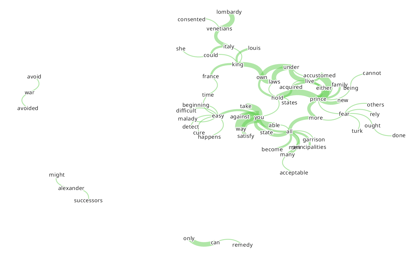
Layouts
Networds use tidygraph and ggraph packages. So, is possible to try
different layouts in the layout parameter. To list the
options available:
layouts
#>  [1] "bipartite" "star"      "circle"    "nicely"    "dh"        "gem"
#>  [7] "graphopt"  "grid"      "mds"       "sphere"    "randomly"  "fr"
#> [13] "kk"        "drl"       "lgl"
Using the nicley layout in the plot:
choosed_layout <- layouts[4]
choosed_layout
#> [1] "nicely"
cooc |>
head(70) |>
dplyr::mutate(n = scale_to_range(n, 0.5, 7)) |>
plot_graph2(Text,
head_n = "", # Run all inputed data, without internal head, let it empty
scale_graph = "", # use no buil-in rescale
edge_color = 3, text_size = 2.5, edge_bend = 0.2,
text_contour_color = "white",
layout = choosed_layout
)
#> You provided a vector of 6 elements instead of one. No problem, but these will be collapsed into a single element, with a final punctuation mark added to each.
#> | | | 0% | |= | 2% | |== | 3% | |=== | 5% | |===== | 7% | |====== | 8% | |======= | 10% | |======== | 11% | |========= | 13% | |========== | 15% | |=========== | 16% | |============= | 18% | |============== | 20% | |=============== | 21% | |================ | 23% | |================= | 25% | |================== | 26% | |==================== | 28% | |===================== | 30% | |====================== | 31% | |======================= | 33% | |======================== | 34% | |========================= | 36% | |========================== | 38% | |============================ | 39% | |============================= | 41% | |============================== | 43% | |=============================== | 44% | |================================ | 46% | |================================= | 48% | |================================== | 49% | |==================================== | 51% | |===================================== | 52% | |====================================== | 54% | |======================================= | 56% | |======================================== | 57% | |========================================= | 59% | |========================================== | 61% | |============================================ | 62% | |============================================= | 64% | |============================================== | 66% | |=============================================== | 67% | |================================================ | 69% | |================================================= | 70% | |================================================== | 72% | |==================================================== | 74% | |===================================================== | 75% | |====================================================== | 77% | |======================================================= | 79% | |======================================================== | 80% | |========================================================= | 82% | |=========================================================== | 84% | |============================================================ | 85% | |============================================================= | 87% | |============================================================== | 89% | |=============================================================== | 90% | |================================================================ | 92% | |================================================================= | 93% | |=================================================================== | 95% | |==================================================================== | 97% | |===================================================================== | 98% | |======================================================================| 100%
#> Using node_size proportional to word frequency as no node_size was provided in parameters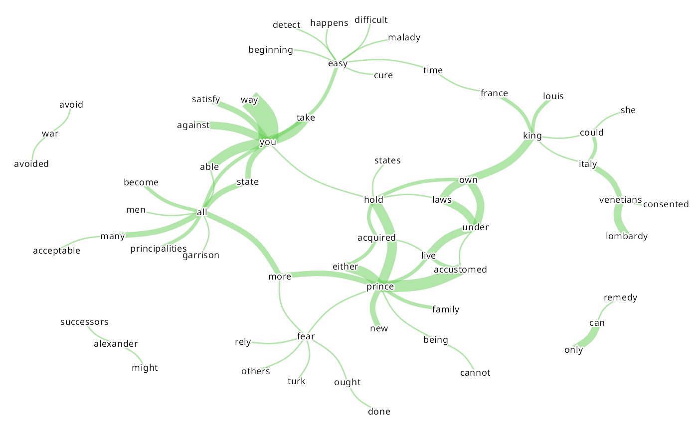
Using the star layout:
choosed_layout <- layouts[2]
choosed_layout
#> [1] "star"
cooc |>
head(50) |>
dplyr::mutate(n = scale_to_range(n, 0.5, 7)) |>
plot_graph2(Text,
head_n = "", # Run all inputed data, without internal head, let it empty
scale_graph = "", # use no buil-in rescale
edge_color = 3, text_size = 2.5, edge_bend = 0.2,
text_contour_color = "white",
layout = choosed_layout
)
#> You provided a vector of 6 elements instead of one. No problem, but these will be collapsed into a single element, with a final punctuation mark added to each.
#> | | | 0% | |= | 2% | |=== | 4% | |==== | 6% | |====== | 9% | |======= | 11% | |========= | 13% | |========== | 15% | |============ | 17% | |============= | 19% | |=============== | 21% | |================ | 23% | |================== | 26% | |=================== | 28% | |===================== | 30% | |====================== | 32% | |======================== | 34% | |========================= | 36% | |=========================== | 38% | |============================ | 40% | |============================== | 43% | |=============================== | 45% | |================================= | 47% | |================================== | 49% | |==================================== | 51% | |===================================== | 53% | |======================================= | 55% | |======================================== | 57% | |========================================== | 60% | |=========================================== | 62% | |============================================= | 64% | |============================================== | 66% | |================================================ | 68% | |================================================= | 70% | |=================================================== | 72% | |==================================================== | 74% | |====================================================== | 77% | |======================================================= | 79% | |========================================================= | 81% | |========================================================== | 83% | |============================================================ | 85% | |============================================================= | 87% | |=============================================================== | 89% | |================================================================ | 91% | |================================================================== | 94% | |=================================================================== | 96% | |===================================================================== | 98% | |======================================================================| 100%
#> Using node_size proportional to word frequency as no node_size was provided in parameters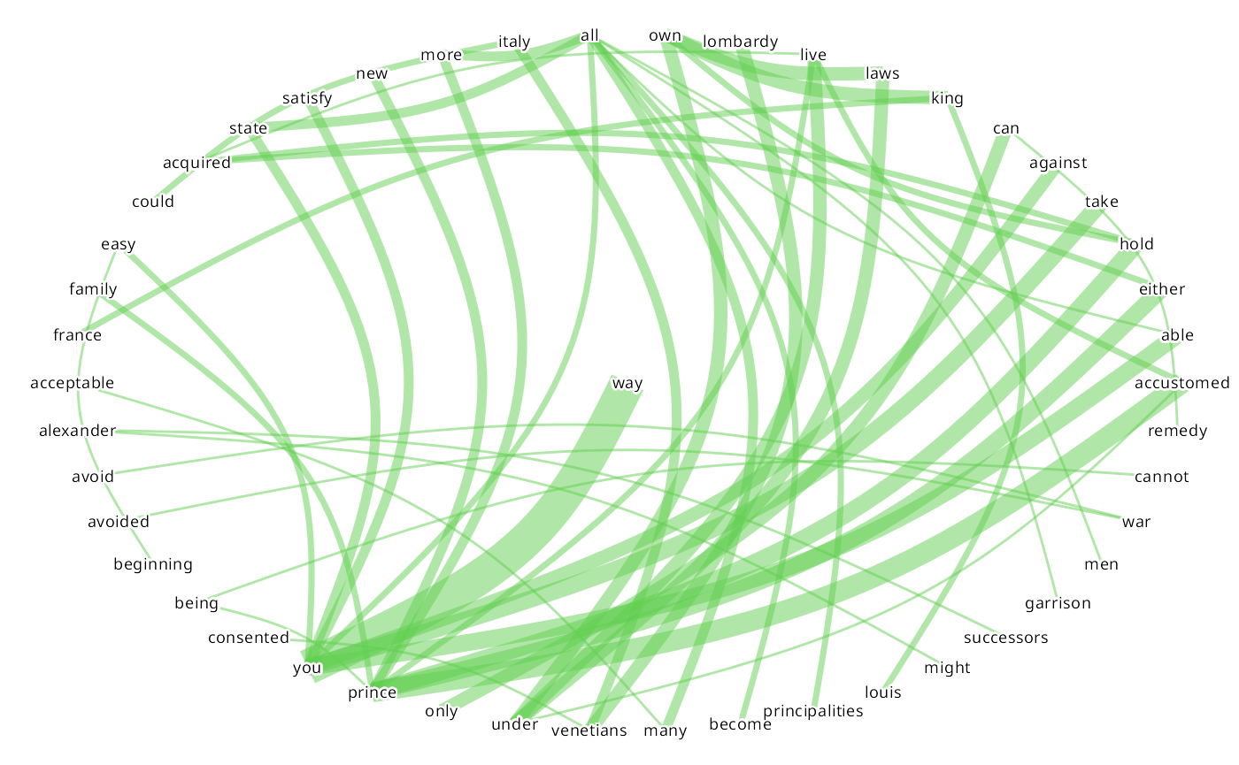
Analysis
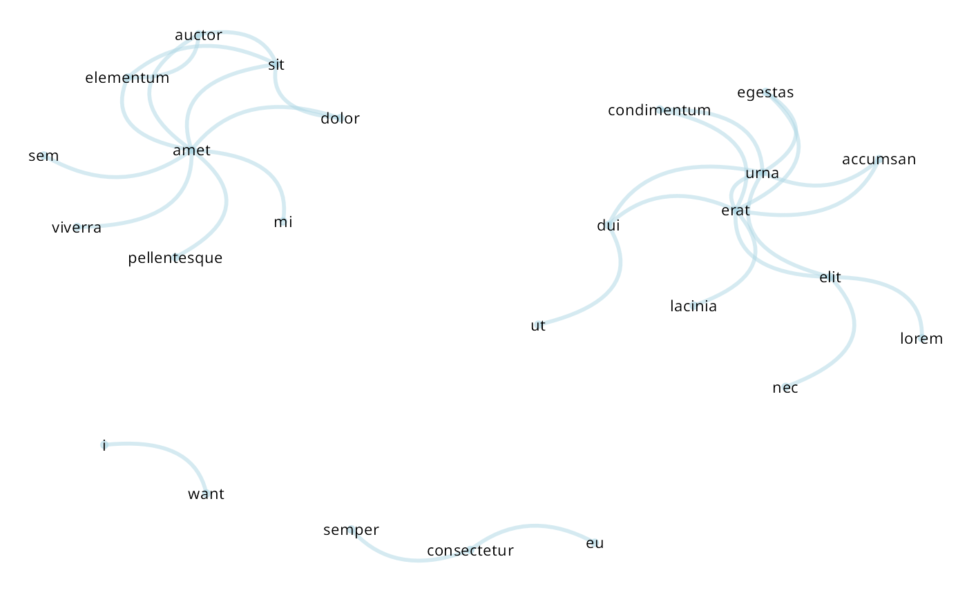
Very dense cluster
Sometimes, we find a very dense cluster of very interconnected node of words. This must sound an alert. Probably is the same chunk of text repeated very often and is only polluting your graph. It can be a good indicator to go back inspect your data and run the coocurrence analysis again.
biased_doc <- "I want apples. I want bananas. I want pineaples. I want avocado."
normal_docs <- c(
  "Lorem ipsum dolor sit amet, consectetur adipiscing elit. Nullam pulvinar ante ut elit scelerisque, nec hendrerit orci dapibus. Ut auctor hendrerit dignissim. Nulla accumsan, lorem non lacinia condimentum, urna dui egestas erat, nec porta urna erat quis elit. ",
  "Aenean consequat molestie est sit amet tincidunt. Pellentesque sit amet dolor auctor, elementum sem sit amet, viverra mi. Aliquam odio magna, auctor in elementum eu, consectetur nec quam. Praesent consectetur tortor massa, semper luctus nulla semper eu. Ut posuere tellus dui, tempor volutpat sem finibus ut."
)

corpus <- c(biased_doc, normal_docs)

cooc <- cooccur_words(corpus)
#> You provided a vector of 3 elements instead of one. No problem, but these will be collapsed into a single element, with a final punctuation mark added to each, to ensure it is treated as different sentences in the process of tokenization.
#> tokenizing sentences...
#> tokenizing words...
cooc |> plot_graph()
#> Only one value passed to edge_width. All edges will have the same width.