Entities and relation extraction
Source:vignettes/entities_and_relation_extraction.Rmd
entities_and_relation_extraction.RmdNamed Entity extraction and its relations
The package {sto} also provides a set of tools to extract entities and relations from text. It does so by one of the simples form: by using the rule based approach. It contains a rule based extraction algorithm and a rule based relation extraction algorithm. For more advanced NER, there is other packages such as {crfsuite}, {UDpipe} and {spacyR}. Another similar package is textnets, from Chris Bail. It capture the proper names using UDpipe, plot word networks and calculates the centrality/betweeness of words in the network.
The functions of {sto} do not work so well like the NER of the mentioned packages, but we think that, in some situations, they can be better job than traditional joining unigram, bigrams, trigrams and so on. Because it is a rule based approach, it is very simple to use, need less dependencies and also fast (or less slower). It will also requires a lot of post-cleaning, but you have the absolute control over which words are extracted and what words are rejected.
In Natural Language Processing, to find proper names or terms that
frequently appears together is called “collocation”, e.g., to find
“United Kingdom”. You can learn more what is collocation and its
statistical details and r function in this article,
and it is also possible to functions like quanteda.textstats::textstat_collocations(),
TextForecast::get_collocations()
to identify them, but it also will require a lot of data cleaning,
specially if you want is proper names.
How it works?
The function captures all words that:
- begins with uppercase,
- followed by other uppercases, lowercase or numbers, without white
space
- it can contain symbols like _, - or
.. - the user can specify a connector, so, words like
“United States of America” are also captured.
In this way, words like “Covid-19” are also captured In languages such as English and Portuguese, it extracts proper names. In German, it also extracts nouns.
There is some trade-off, of course. It will capture a lot of
undesired words and will demand posterior cleaning, like:
- It does not contain any sort of built-in classification.
- “Obama Chief of Staff Rahm Emanuel” will be captured as one entity,
what is not wrong et al, but maybe not what was expect.
The downsides are
It will not capture: - entities that begin with lowercase. To do that, take a look at other already mentioned packages, like spacyr and UDpipe.
In my experience, this approach works better to certain types of text than others. Books, formal articles can be a good option that works well with this function. Text from social media, because it lacks formalities of the language and have a lot of types, it will not work so well.
So, let’s extract some proper names from a simple text:
"John Does lives in New York in United States of America." |> extract_entity()
#> [1] "John Does"                "New York"
#> [3] "United States of America"
Or it is possible to use other languages, specifying the parameter
connectors using the function
connectors(lang). Checking the connectors:
connectors("eng")
#> [1] "of"     "of the"
connectors("pt")
#> [1] "da"  "das" "de"  "do"  "dos"
connectors("port")
#> [1] "da"  "das" "de"  "do"  "dos"

# by default, the functions uses the parameter "misc". meaning "miscellaneous".
connectors("misc")
#> [1] "of"     "the"    "of the" "von"    "van"    "del"
Using with other languages:
"João Ninguém mora em São José do Rio Preto. Ele esteve antes em Sergipe" |>
  extract_entity(connect = connectors("pt"))
#> [1] "João Ninguém"          "São José do Rio Preto" "Ele"
#> [4] "Sergipe"

vonNeumann_txt <- "John von Neumann (/vɒn ˈnɔɪmən/ von NOY-mən; Hungarian: Neumann János Lajos [ˈnɒjmɒn ˈjaːnoʃ ˈlɒjoʃ]; December 28, 1903 – February 8, 1957) was a Hungarian and American mathematician, physicist, computer scientist and engineer"
vonNeumann_txt |> extract_entity()
#> [1] "John von Neumann"    "NOY-"                "Hungarian"
#> [4] "Neumann János Lajos" "December"            "February"
#> [7] "Hungarian"           "American"
Extracting a graph
It is possible to extract a graph from the extracted entities. First,
happens the tokenization by sentence or paragraph. Than, the entities
are extracted using extract_entity(). Than a data frame
with the co-occurrence of words in sentences or paragraph is build.
vonNeumann_txt |> extract_graph()
#> Tokenizing by sentences
#> # A tibble: 27 × 2
#>    n1               n2
#>    <chr>            <chr>
#>  1 John von Neumann NOY-
#>  2 John von Neumann Hungarian
#>  3 John von Neumann Neumann János Lajos
#>  4 John von Neumann December
#>  5 John von Neumann February
#>  6 John von Neumann Hungarian
#>  7 John von Neumann American
#>  8 NOY-             Hungarian
#>  9 NOY-             Neumann János Lajos
#> 10 NOY-             December
#> # ℹ 17 more rows
This process can take a while to run if the text/corpus is big. So, if you are interested only in some words, so first of all, filter the sentences/paragraphs with the desired words, and after that, extract the graph. Seeing another example, extracting from a wikipedia article:
page <- "https://en.wikipedia.org/wiki/GNU_General_Public_License" |> rvest::read_html()
text <- page |>
  rvest::html_nodes("p") |>
  rvest::html_text()
# looking at the scraped text:
text[1:2] # seeing the head of the text
#> [1] "\n\n"
#> [2] "The GNU General Public Licenses (GNU GPL, or simply GPL) are a series of widely used free software licenses, or copyleft licenses, that guarantee end users the freedoms to run, study, share, or modify the software.[7] The GPL was the first copyleft license available for general use. It was originally written by Richard Stallman, the founder of the Free Software Foundation (FSF), for the GNU Project. The license grants the recipients of a computer program the rights of the Free Software Definition.[8] The licenses in the GPL series are all copyleft licenses, which means that any derivative work must be distributed under the same or equivalent license terms. It is more restrictive than the Lesser General Public License, and even further distinct from the more widely used permissive software licenses such as BSD, MIT, and Apache.\n"
And now extracting the graphs:
g <- text |> extract_graph(sw = gen_stopwords("en", add = "The This It"))
#> Tokenizing by sentences
g
#> # A tibble: 3,891 × 2
#>    n1                              n2
#>    <chr>                           <chr>
#>  1 The GNU General Public Licenses GNU GPL
#>  2 The GNU General Public Licenses GPL
#>  3 The GNU General Public Licenses The GPL
#>  4 The GNU General Public Licenses Richard Stallman
#>  5 The GNU General Public Licenses Free Software Foundation
#>  6 The GNU General Public Licenses FSF
#>  7 The GNU General Public Licenses GNU Project
#>  8 The GNU General Public Licenses Free Software Definition
#>  9 The GNU General Public Licenses GPL
#> 10 The GNU General Public Licenses Lesser General Public License
#> # ℹ 3,881 more rows
g_N <- g |> dplyr::count(n1, n2, sort = T)
g_N
#> # A tibble: 2,550 × 3
#>    n1           n2               n
#>    <chr>        <chr>        <int>
#>  1 In           GPL             32
#>  2 GPLv3        GPLv2           25
#>  3 Artifex      Hancom          19
#>  4 Ghostscript  Hancom          19
#>  5 GPL-licensed GPL             17
#>  6 GPL          GPL-licensed    16
#>  7 GPL          GPLv3           14
#>  8 GPL          FSF             13
#>  9 GPLv2        GPLv3           13
#> 10 Linux        GPL             13
#> # ℹ 2,540 more rows
plot_graph(text, g_N)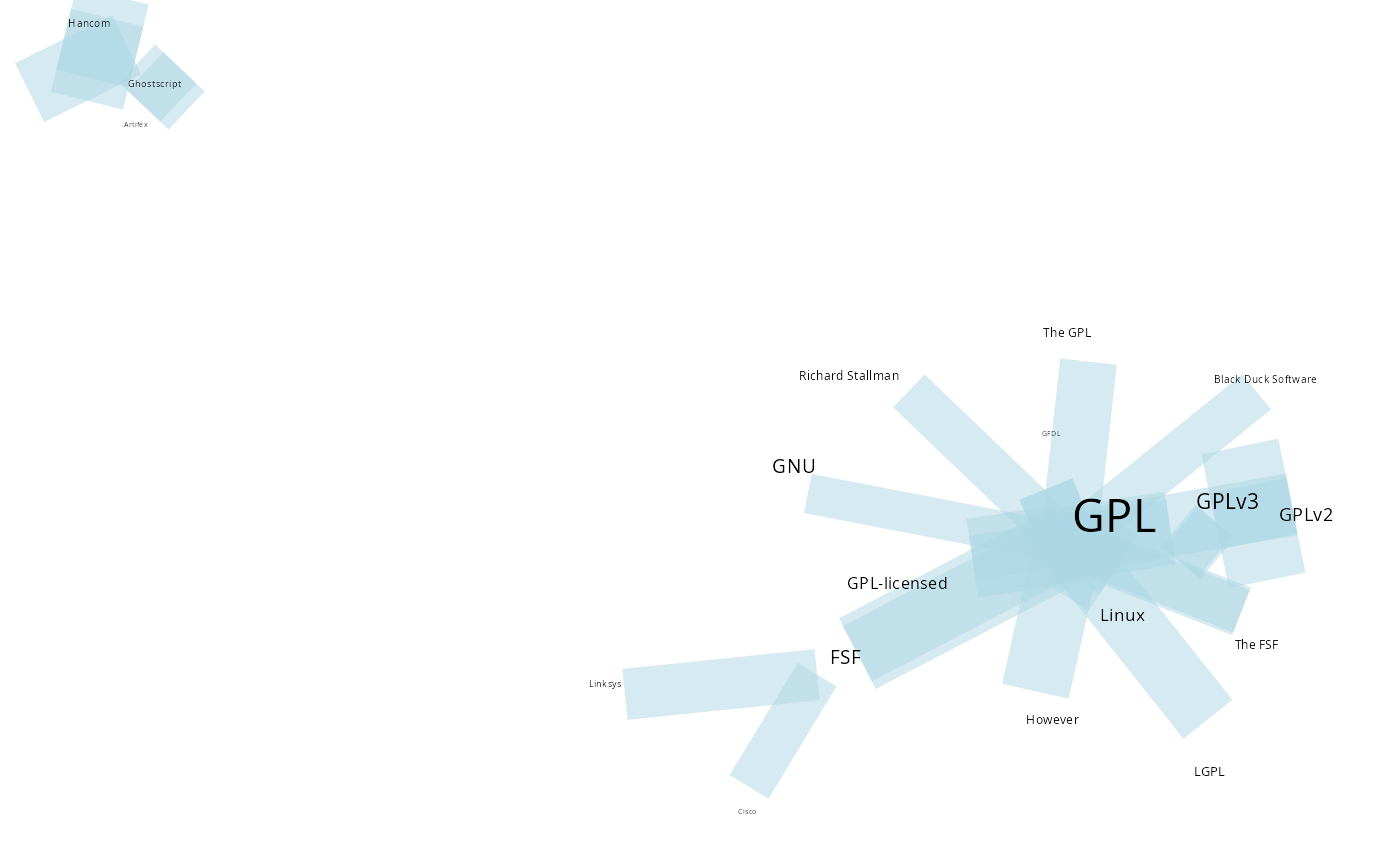 There are different information in the graph - The size of words and
compound words means the individual frequency of each one - The
thickness of the links indicates how often the pair occur together.
There are different information in the graph - The size of words and
compound words means the individual frequency of each one - The
thickness of the links indicates how often the pair occur together.
To plot an interactive graph, it is possible to use {networkD3}:
g_N |>
  head(100) |> # to reduce the amount of nodes and edges in the graph
  networkD3::simpleNetwork(
    height = "10px", width = "30px",
    linkDistance = 50,
    fontSize = 16
  )
Another text example.
page <- "https://en.wikipedia.org/wiki/Hurricane_Milton" |> rvest::read_html()
text <- page |>
rvest::html_nodes("p") |>
rvest::html_text()
text[1:2] # seeing the head of the tex
#> [1] "\n" "\n\n"
g <- text |> extract_graph(sw = gen_stopwords("en", add = "The This It"))
#> Tokenizing by sentences
g_N <- g |> dplyr::count(n1, n2, sort = T)
plot_graph(text, g_N, head_n = 50)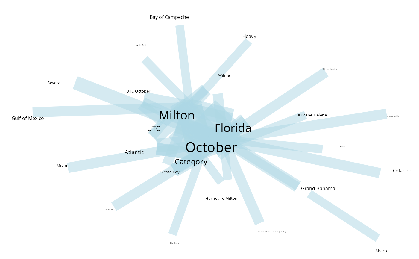 To plot an interactive graph, it is possible to use {networkD3}:
g_N |>
  head(100) |> # to reduce the amount of nodes and edges in the graph
  networkD3::simpleNetwork(
    height = "10px", width = "30px",
    linkDistance = 50,
    fontSize = 16
  )